Goldman Sachs Research
Global Economics Analyst
Our New G10 Financial Conditions Indices
20 April 2017 | 2:26PM EDT | Research | Economics| By Jan Hatzius and others
More
  • We have unified our financial conditions indices (FCIs) for the G10 economies using models that are methodologically consistent with one another while still allowing for structural differences between the economies. All ten FCIs are updated daily, and are published on Bloomberg.

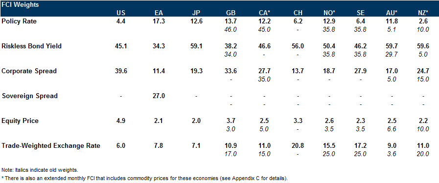
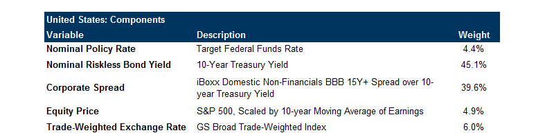
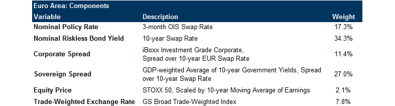
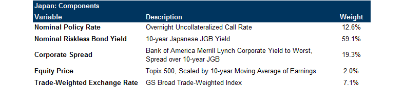
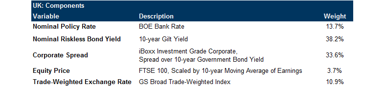
  • Each FCI is calculated as a weighted average of a policy rate, a long-term risk-free bond yield, a corporate credit spread, an equity price variable, and a trade-weighted exchange rate; in the Euro area we also include a sovereign credit spread. The weights mirror the effects of the financial variables on real GDP growth in our models over a one-year horizon.

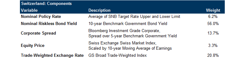
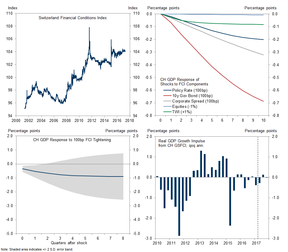
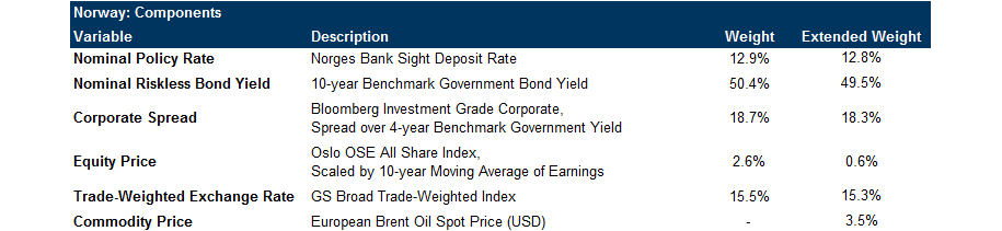
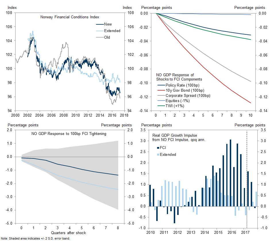
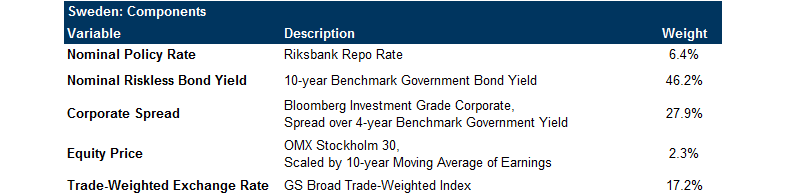
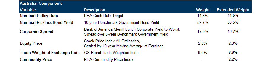
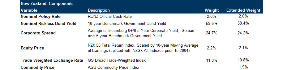
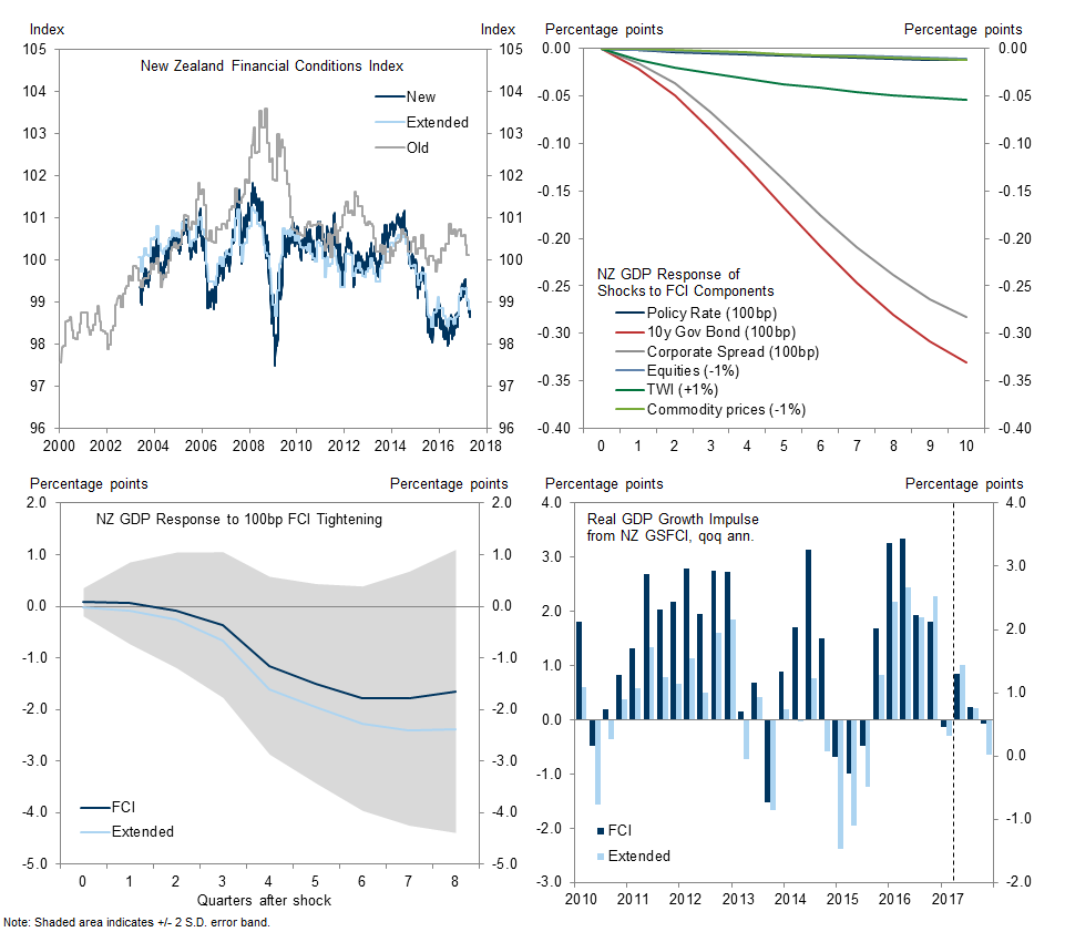
  • The FCIs for the US, Euro area and Japan are unchanged from their recent revamp but we made a number of significant changes to the other G10 FCIs. The updated FCIs now generally have a smaller weight on the policy rate, a bigger weight on long-term interest rates and corporate spreads, and a smaller weight on the exchange rate. The FCIs for Australia and New Zealand no longer contain commodity and house prices. But we now also provide extended monthly measures that contain commodity prices for Australia, New Zealand, Canada and Norway. We produce an FCI for Switzerland for the first time.

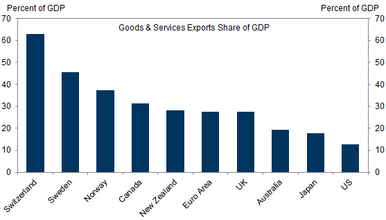
  • Differences in weights across economies reflect differences in financial systems and economic structures. Economies with larger shares of variable-rate borrowing also have larger weights on short-term rates. Similarly, equity prices and corporate credit spreads generally have the biggest weights in countries where these markets are more common sources of firms’ funding. The exchange rate is much more important in the small open economies than in the US.

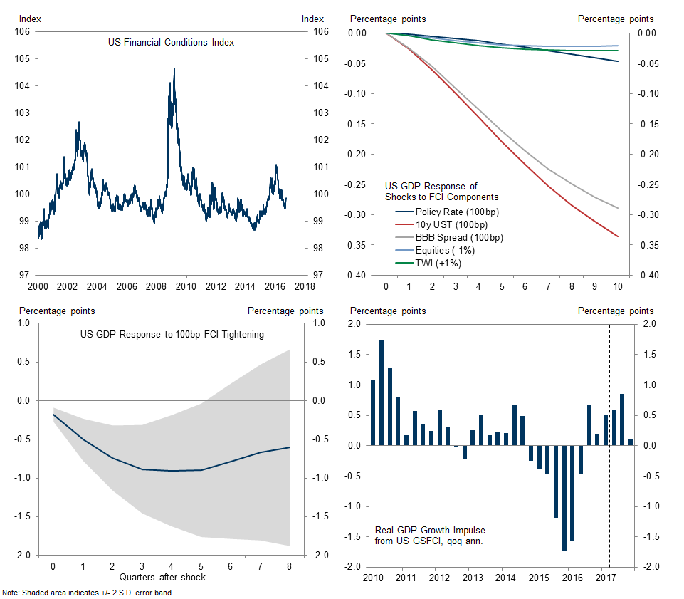
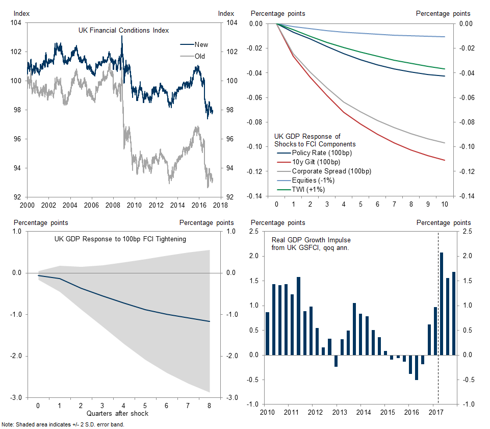
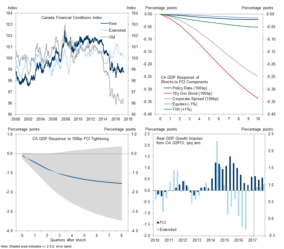
  • Our revised FCIs have meaningful predictive power for growth, especially in the large G10 economies. We find that financial conditions have played an important role in supporting the recent pickup of growth across the advanced economies. The FCI impulse is currently most positive in the US, UK, Sweden and Norway; it is more neutral in Australia, New Zealand, Japan and Switzerland. Our estimates point to a continued boost from financial conditions this year, consistent with our expectation of above-trend growth in most G10 economies.

We have long emphasized the importance of financial conditions for the economic and monetary policy outlook, and have therefore developed financial conditions indices (FCIs) for each of the world’s large economies as well as many smaller ones.[1] Last year we revamped the FCIs of the US, Euro area and Japan to make them easily comparable, by adopting the same broad modelling structure for each.[2] This brought the benefit of using a consistent model, but with enough flexibility to allow for structural differences among the economies. Today we extend this new approach to the remaining G10 economies, namely the UK, Canada, Australia, New Zealand, Sweden, Norway, and Switzerland.
We update all ten FCIs on a daily basis, and publish the data on Bloomberg. The tickers are reported in Appendix A below.

Our New FCIs

Exhibit 1 plots our new G10 FCIs against the prior versions. The US, Euro area and Japan FCIs are unchanged from their recent update, but some of the other G10 FCIs now look quite different. Exhibit 2 shows how the weights have changed from the prior version. The box on page 5 provides an overview of the input variables. Appendix B discusses the underlying econometric models and Appendix C provides a detailed description of the variables used in each country.
We make the following changes to our FCIs in the smaller G10 economies:
  • Most importantly, we now apply the same modeling approach across all economies, to estimate the partial impact of changes in each financial variable while holding the other variables constant. This avoids giving too much weight to some variables—such as the short-term policy rate—whose effect on GDP actually comes via their impact on other series such as long-term yields and the exchange rate.

  • Corporate credit spreads are now included in all economies. Incorporating credit measures is particularly important for the US and UK, where credit risk has played an important role in the business cycle in recent years.

  • We now scale equity prices by a 10-year moving average of earnings. This eliminates the artificial trend toward a higher equity variable and easier financial conditions that results from using a nominal equity price index.

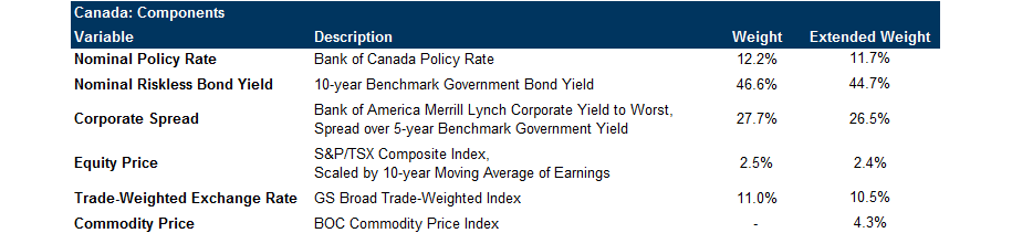
  • To make the daily FCIs comparable across countries, we exclude commodity and house prices from all series. This affects the old Australia and New Zealand FCIs, but sharpens the focus towards purely financial variables for day-to-day moves in financial conditions. But since commodity prices are particularly relevant to Canada, Norway, Australia, and New Zealand, we also produce an extended FCI at monthly frequency, which incorporates relevant commodity prices for each.[3]

Exhibit 1: Our New G10 FCIs

1. Our New G10 FCIs. Data available on request.
Source: Goldman Sachs Global Investment Research

 . Data available on request.
Source: Goldman Sachs Global Investment Research

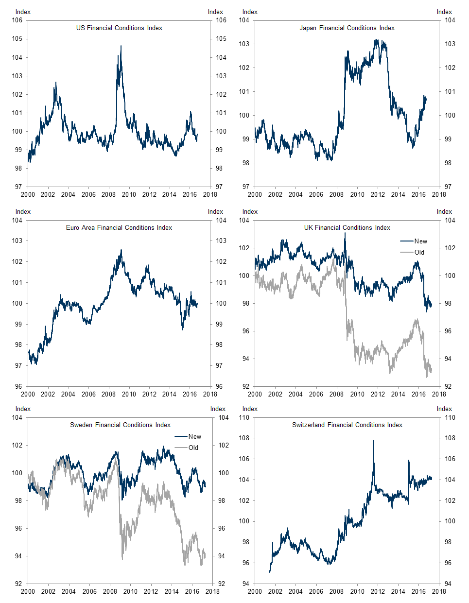
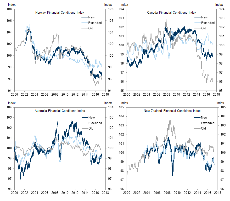
Exhibit 2: New vs. Old Weights

2. New vs. Old Weights. Data available on request.
Source: Goldman Sachs Global Investment Research
Box: Data description
The FCI components generally cover six areas, although the precise setup for each economy depends on its structure. Details of all the components are listed by country in Appendix C, so this box provides a high-level overview.
  • Interest rates. We use the policy rate and the nominal 10-year risk-free rate.

  • Corporate spread. We use investment-grade domestic corporate spreads over equivalent-duration government bond yields.

  • Sovereign spread. For the Euro area we also include a measure of sovereign risk within the bloc, by including GDP-weighted 10-year government yields, and take the spread of this over the 10-year swap rate.

  • Equity prices. To get a stationary series for equity prices, we use the ratio of a broad-based equity index to a lagged 10-year average of earnings per share, which has become known as the “Shiller P/E” ratio.

  • Commodity prices. To reflect the importance of commodity prices in Canada, Norway, Australia, and New Zealand, we also include commodity prices in an extended monthly FCI. The daily FCI series for all G10 countries focus solely on financial series, and exclude commodity prices.

  • Trade-weighted exchange rate. We use the broad GS nominal trade-weighted exchange rate index. This is the trade-weighted average of 36 bilateral exchange rates, with weights that reflect each economy’s exports, imports and third-market competition of domestic firms vis-à-vis foreign firms.

Our daily GSFCIs with the variables above start in the early 2000s, and we set them equal to 100 for the average since 2000 (or the first data point, if later). Deviations of the GSCFIs from 100 show how far financial conditions have deviated from “normal” during this period.

Different Weights for Different Economies

Given our common approach, we can relate differences in the weight of a particular variable across economies to differences in economic or financial structure. Three points are worth noting here.
1. Policy rates. The weight on the policy rate in all economies (except Australia) is now smaller than in the previous version of our FCIs. But there are still wide variations in the weight, which partly reflects differences in the share of short-term borrowing, as illustrated in Exhibit 3. It may also reflect the fact that banks—which typically benefit from a lower policy rate because it tends to steepen the yield curve and increase net interest income—play a more important role in some financial systems, such as Europe and Japan, than in the US.[4]

Exhibit 3: More Variable Rate Mortgages in Europe and Australia

3. More Variable Rate Mortgages in Europe and Australia. Data available on request.
Source: Badarinza et al (2014), Lea (2010), Bank of Canada, Bank of England
2. Equity and corporate credit markets. The weight on equity prices and corporate credit spreads is relatively large in the US, where these markets are more central for consumers and businesses than elsewhere. Exhibit 4 shows the share of household wealth held in equities for a range of countries, and illustrates the wide range of variation between them. Moreover, Exhibit 5 shows that US corporations obtain a much larger share of their borrowing from the bond and commercial paper markets than corporations in the other G10.

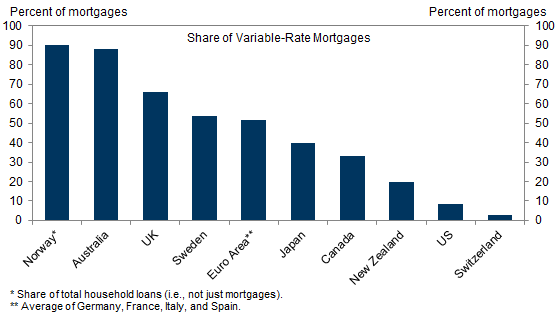
Exhibit 4: The Importance of Equities in Total Household Wealth Varies Markedly Across Countries

4. The Importance of Equities in Total Household Wealth Varies Markedly Across Countries. Data available on request.
Source: OECD

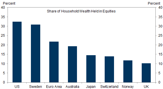
Exhibit 5: Corporate Borrowing From Bond Markets vs. Banks

5. Corporate Borrowing From Bond Markets vs. Banks. Data available on request.
Source: Federal Reserve Board, European Central Bank, Bank of Japan, Goldman Sachs Global Investment Research
3. Exchange rates. While the equity and credit markets are more important in the US than elsewhere, the exchange rate is less important because the US is less dependent on foreign trade than other economies. Exhibit 6 shows that exports as a share of GDP are only 13% for the US, compared, for example, with 28% for the Euro area or 63% for Switzerland.

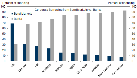
Exhibit 6: Smaller Economies Also Tend to Be More Open

6. Smaller Economies Also Tend to Be More Open. Data available on request.
Source: International Monetary Fund, Goldman Sachs Global Investment Research

Weights vs. Importance

The importance of our financial variables for financial conditions depends not just on the weights of the different variables shown in Exhibit 2 but also on their volatility. For example, while the long-term risk-free bond yield has a much higher weight than the equity market or the trade-weighted exchange rate, it also moves around a lot less, so it is not obvious which variable is more important. To get a better sense of relative importance, Exhibit 7 shows the average contributions of the absolute annual changes in each component, since 2000.

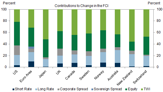
Exhibit 7: Exchange Rates and Equities Drive Most of FCI Changes

7. Exchange Rates and Equities Drive Most of FCI Changes. Data available on request.
Source: Goldman Sachs Global Investment Research
The results show that the currency and equity markets have a substantially greater impact on our FCIs than suggested by the relatively small weights in Exhibit 2. The equity market is particularly important in the US, while the currency markets are more important elsewhere, such as Japan, New Zealand and Switzerland. Bond markets and credit spreads are also important, but generally less so than one might think based only on their relatively large weights in Exhibit 2. The disconnect is more pronounced for Japan, possibly reflecting the fact that short and long rates have been more constrained by the zero lower bound than in the US and Euro area.

The Link with Growth

Our revised FCIs have meaningful predictive power for growth, although the extent varies across countries. We construct a simple vector autoregression model for each country to estimate the impact of a 100bp FCI tightening on real GDP.[5] Exhibit 8 shows the impulse responses for the US, Euro area, Japan and the UK. Appendix C provides details for each country. The effects build gradually over the first year before generally leveling off in the second year. The effect of a 100bp FCI tightening is around 0.9pp in the US, 0.8 in the Euro area, and 0.7pp in Japan. The impact is statistically significant at the 5% level in the US and Japan, and at the 10% level in the Euro area and the UK.

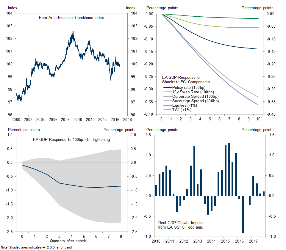
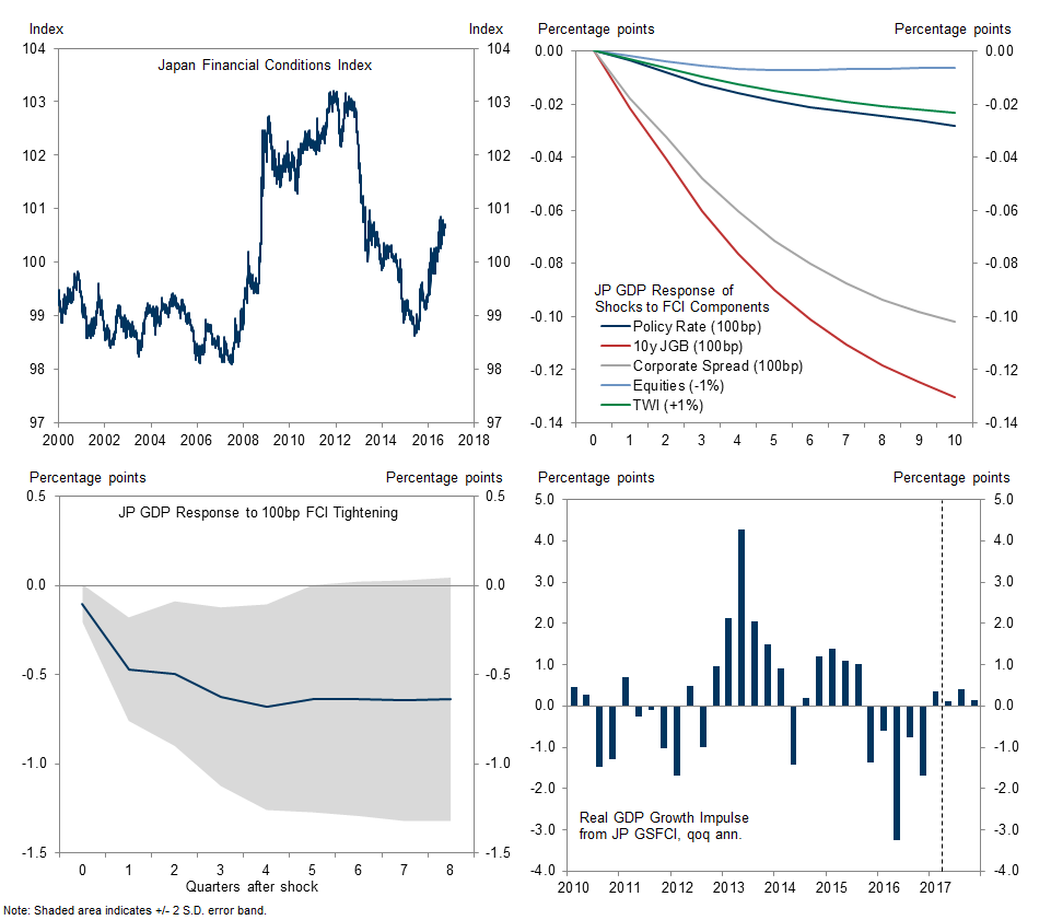
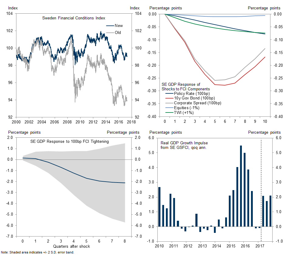
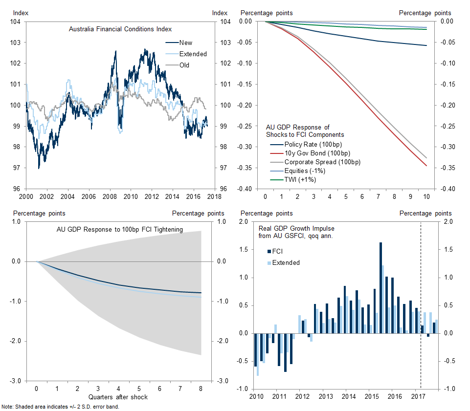
Exhibit 8: G4 Impulse Responses

8. G4 Impulse Responses. Data available on request.
Source: Goldman Sachs Global Investment Research
Exhibit 9 shows a summary of the four-quarter effects for all G10 economies. The one-year impact of a 100bp tightening on real GDP growth after one year clusters around 0.9pp across the G10 economies. The estimated growth effects of financial shocks tend to be less precisely estimated in the smaller G10 economies.
We can use these VARs to generate an “FCI impulse” for each G10 economy, defined as the effect of lagged financial conditions shocks on GDP growth. This impulse provides a summary of how financial conditions are influencing growth at any point in time.[6] Exhibit 10 provides a summary of the FCI impulses across the G10 since 2014. The Appendix provides additional details for how we calculate the FCI impulses and shows the results for each of the ten economies.

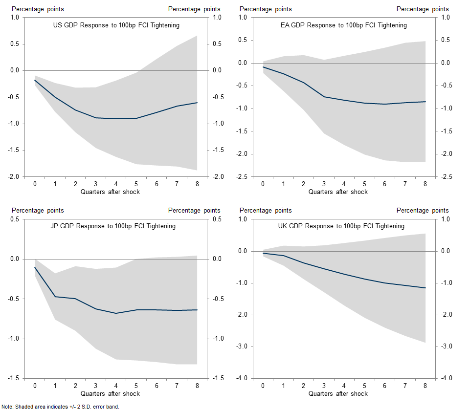
Exhibit 9: Impact of a 100bp FCI Tightening Varies Across Countries

9. Impact of a 100bp FCI Tightening Varies Across Countries. Data available on request.
Source: Goldman Sachs Global Investment Research
Our estimates show that the FCI impulses across the G10 have generally turned more positive over the last year. Financial conditions acted as a drag across the big four G10 economies in late 2015/early 2016, but then swung to a boost in late 2016. Our estimates suggest that financial conditions will boost G4 growth by an average of 1/2pp this year, before beginning to fade next year. The FCI impulse is most positive in the UK (due to the sharp depreciation of Sterling after the EU referendum) and the US.[7] Financial conditions are only somewhat supportive for growth in the Euro area and Japan this year.

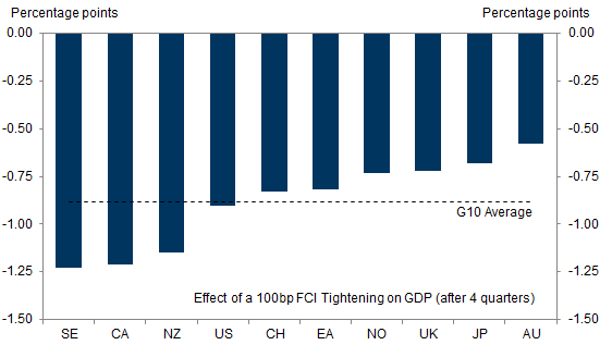
Exhibit 10: FCI Impulses Have Turned Positive

10. FCI Impulses Have Turned Positive. Data available on request.
Source: Goldman Sachs Global Investment Research
The FCI impulses are also positive in the smaller G10 economies, except in Switzerland. Conditions are particularly growth supportive in Sweden, due to the effects of highly expansionary monetary policies. The FCI impulse in Switzerland has generally been negative in recent years, given the strength of the Swiss Franc.

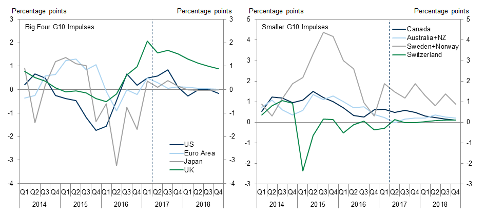
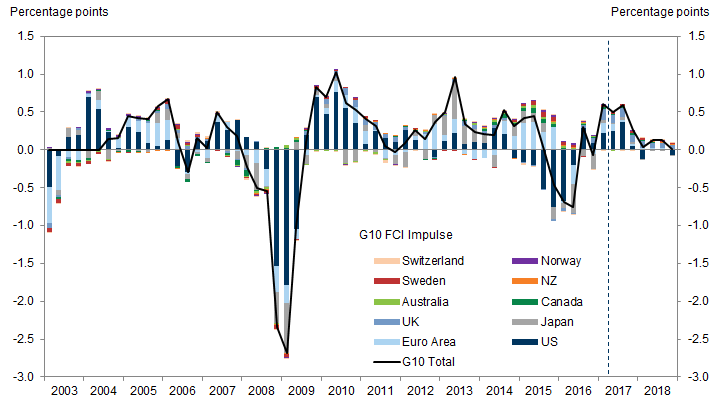
Exhibit 11: A G10 FCI Impulse

11. A G10 FCI Impulse. Data available on request.
Source: Goldman Sachs Global Investment Research
Exhibit 11 aggregates the individual impulses to a G10 FCI impulse. We see that financial conditions have played an important role in supporting the pickup of growth across the advanced economies since last summer. The G10 FCI impulses point to a continued boost from financial conditions this year, consistent with our expectation of above-trend growth in most advanced economies.

Nicholas Fawcett

Sven Jari Stehn

Jan Hatzius

 . Data available on request.

Appendix A: Bloomberg Tickers

 . Data available on request.
Source: Goldman Sachs Global Investment Research

Appendix B: Building a Unified Framework for Financial Conditions

Model details
Our stylized macro models are broadly the same for all G10 economies and similar to the models we have used in recent research.[8] We specify a set of long-run behavioral relationships that link the components of GDP to some underlying drivers. This partly determines short-run movements in the model, as each component tends back towards its long-run equilibrium relationship; recent dynamics also explain changes in the short run.
Long-run consumption (Ct) is determined by real disposable income (Ydt) and wealth (Wet).[9] For the US and Euro area models, total wealth is broken down into equity and housing components, and for other economies where consistent equity wealth data are unavailable, we use real equity prices:

 . Data available on request.
Non-residential investment as a share of potential GDP (INRt) is driven by real corporate borrowing costs. This is measured by combining the 10-year government safe rate (rlt) with a corporate borrowing spread (spreadt). In the Euro area model, we also find that the ratio of equity prices to nominal GDP is an important determinant, and for Australia and New Zealand we include commodity prices deflated by the GDP deflator.

 . Data available on request.
There are substantial differences in the sources of funding for firms across the economies. For example, Euro area firms make more extensive use of bank loan financing than US firms; the latter make greater use of corporate debt markets. To account for this, our corporate spread variable incorporates a blend of different borrowing costs, with weights depending on the economy.
Residential investment (IRt/Y*t) is driven by a weighted average of real short-term (rst) and long-term interest rates and the growth rate of potential GDP (gt):

 . Data available on request.
The trade equations are similar for both imports (Mt) and exports (Xt). The two are modelled as shares of domestic and trade-weighted world demand respectively, and depend on the real effective exchange rate (RERt). We allow for deterministic trends in both long-run relationships, to capture structural changes in world trade, for example caused by globalization.

 . Data available on request.
GDP is then determined as the sum of the projections of these components.
Table 1 reports the values of key parameters in the equations above for each of the economies. Some of these parameters are estimated, using quarterly data, while others are known to be hard to pin down directly--in particular the sensitivity of investment to interest rates, and the sensitivity of trade flows to the exchange rate. We have therefore calibrated these parameters based on our previous work,[10] our reading of the academic literature and existing country models.

Table 1: Comparison of Model Parameters Across Economies

Table 1: Comparison of Model Parameters Across Economies. Data available on request.
Source: Goldman Sachs Global Investment Research

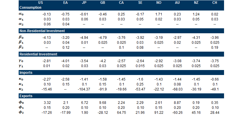
Simulating the effect of FCI component shocks

We shock each of the FCI components separately to compare their effect on GDP. This comparison generates the component weights in the overall FCI. In order to isolate the impact of each component on the model, we proceed as follows: we introduce a permanent shock to one component (a 100bp increase for interest rates and spreads, a 1% fall in equities, and a 1% rise in the TWI, and for the monthly extended FCIs, a 1% rise in commodity prices) but hold all other financial variables constant. This gives the cleanest estimate of the direct impact of that component on activity, without inadvertently double-counting effects that come through the other financial variables.
The country-by-country charts in the Appendix trace out this exercise for each economy. A permanent 100bp shock to the long-term safe rate, for example, triggers a fall in GDP three years later of just under 0.4% in the US, around 0.4% in the Euro area and around 0.14% in Japan. By contrast, a permanent 10% fall in equity prices leads to a fall in GDP of between 0.1% and 0.2% in all three economies.
We then use the GDP effect four quarters after the shock to calculate the weight of each component in the FCI. So the fact that, for the US, the impact of a shock to the 10-year Treasury yield is nearly seven times as big as the impact of a shock to the exchange rate means that its weight should be nearly seven times as big.

From model weights to FCI weights

Some of the financial variables in our economic models differ from those in our FCI. This affects the equity variable, and some of the elements in the corporate spread. To map from the model spread components to the FCI spreads detailed in the box on page 5, we relate the former to the latter using a simple regression for each country and find that there is a strong relationship between the two. The estimated link also allows us to translate the model weights into FCI weights for the corporate spread. The equity weight is scaled by the relative volatility of the model equity indices and the equity series used in the FCI. The overall component weights are then normalized to ensure they sum to one.

Constructing FCI Impulse

The FCI impulse is designed to measure the contribution of current and past financial conditions on real GDP growth. It is calculated in four steps:
First, we estimate a statistical model linking changes in financial conditions and real GDP growth. This vector autoregression model (VAR) comprises changes in the FCI and qoq annualized real GDP growth, and—for smaller economies more open to trade—trade-weighted foreign demand and—for commodity producers—commodity prices.[11] The models use quarterly data, and the sample period and number of lags differ across countries.
Second, we make assumptions on the order in which financial conditions and growth respond to each other. We identify the VAR using a Cholesky decomposition. As it is difficult to take a strong view on the ordering, we consider two orderings, one in which the FCI appears before GDP, and vice versa, holding the position of any other elements of the VAR unchanged.[12] The impulse responses show a significant effect of shocks to financial conditions on real GDP for either ordering.
Third, we make assumptions for financial conditions going forward. Specifically, we assume that the FCI remains at its current (daily) level until the end of the forecast horizon. We also use the VAR to generate a baseline projection for real GDP growth over this horizon.
Fourth, we use statistical techniques to calculate the historical and projected FCI impulse. We decompose historical and projected real GDP growth into contributions from FCI and growth using the structural shocks calculated in step two above. We calculate the impulse for each of the two possible orderings and define the average as our FCI impulse.

Appendix C: Country details

 . Data available on request.
Source: Goldman Sachs Global Investment Research

 . Data available on request.
Source: Goldman Sachs Global Investment Research

 . Data available on request.
Source: Goldman Sachs Global Investment Research

 . Data available on request.
Source: Goldman Sachs Global Investment Research

 . Data available on request.
Source: Goldman Sachs Global Investment Research

 . Data available on request.
Source: Goldman Sachs Global Investment Research

 . Data available on request.
Source: Goldman Sachs Global Investment Research

 . Data available on request.
Source: Goldman Sachs Global Investment Research

 . Data available on request.
Source: Goldman Sachs Global Investment Research

 . Data available on request.
Source: Goldman Sachs Global Investment Research

 . Data available on request.
Source: Goldman Sachs Global Investment Research

 . Data available on request.
Source: Goldman Sachs Global Investment Research

 . Data available on request.
Source: Goldman Sachs Global Investment Research

 . Data available on request.
Source: Goldman Sachs Global Investment Research

 . Data available on request.
Source: Goldman Sachs Global Investment Research

 . Data available on request.
Source: Goldman Sachs Global Investment Research

 . Data available on request.
Source: Goldman Sachs Global Investment Research

 . Data available on request.
Source: Goldman Sachs Global Investment Research

 . Data available on request.
Source: Goldman Sachs Global Investment Research

 . Data available on request.
Source: Goldman Sachs Global Investment Research
  1. 1 ^ See William C. Dudley and Jan Hatzius, “The Goldman Sachs Financial Conditions Index: The Right Tool for a New Monetary Policy Regime,” Global Economics Paper No. 44, June 8, 2000.
  2. 2 ^ See Jan Hatzius, Sven Jari Stehn and Nicholas Fawcett, “Financial Conditions: A Unified Approach,” Global Economics Analyst, September 20, 2016.
  3. 3 ^ Details of the commodity series are included in Appendix C. Some of these series are composite measures weighted by commodity production, rather than consumption; but although the path of commodity prices obtained by the former rather than the latter may differ at times, the gap is unlikely to be systematically big.
  4. 4 ^ Admittedly, the direct effect of policy rate cuts may be smaller if rates are already negative and banks are unable to pass through additional cuts to their depositors. Even if that is the case, however, the distortions to the FCI would be small. For example, the weight of the policy rate in Japan is 12%, so that a 10bp rate cut eases our FCI directly by only 1.2bp. And if it is true that negative policy rates hurt the economy, as some believe, this would presumably show up in tighter conditions via the FX or equity markets, which we do pick up. A good example is the January 2016 BoJ cut, which was followed by a meaningful tightening in the Japan FCI.
  5. 5 ^ The VARs use quarterly data and include only the FCI and real GDP in the US, Euro area and Japan. In the smaller G10 economies we also include a measure of foreign demand in the VAR (except in Australia). In the commodity-producing economies (Australia, New Zealand, Canada and Norway) we also include measures of commodity prices. Since it is not clear theoretically how to order the variables when computing the impulse responses—as causation within a given quarter likely runs in both directions—Exhibit 8 shows an average of the impulse responses for two different orderings (one orders GDP before the FCI; the other orders the FCI before GDP growth). We order the FCIs last in Australia and Switzerland.
  6. 6 ^ This summary is specific to the setup of the model. Of course, growth will be affected by other factors--such as fiscal policy--which we do not capture explicitly in the model.
  7. 7 ^ The projected UK FCI impulse comes with the caveat that the model does not take into account the impact of greater uncertainty in the UK surrounding the EU referendum, or our UK economists' view that higher inflation will weigh on real disposable incomes, both of which could drag on growth.
  8. 8 ^ See, for example, “Japan’s Easing Options,” Global Economics Analyst, July 27, 2016; and “The Bank of England’s Trade-off,” Global Economics Analyst, August 2, 2016.
  9. 9 ^ We also include an aging variable in Japan to capture demographic changes.
  10. 10 ^ See “How much does the exchange rate matter for growth?”, Global Economics Analyst, 10 September 2016.
  11. 11 ^ We do not include foreign demand in the Australia VAR.
  12. 12 ^ We order the FCI last in Australia and Switzerland.

Investors should consider this report as only a single factor in making their investment decision. For Reg AC certification and other important disclosures, see the Disclosure Appendix, or go to www.gs.com/research/hedge.html.