Goldman Sachs Research
Global Markets Analyst
Distilling Macro Themes from Market Prices
8 October 2018 | 12:38AM EDT | Research | Economics| By Charles P. Himmelberg and others
More
  • A big macro week in markets. Macro market volatility jumped last week, with the 10-year Treasury yield jumping 17 bps to close the week at 3.23% (its highest level since 2011), and Brent oil prices rising $3.57 at midweek before closing the week $1.44 higher at $84.26 (its highest level since 2014). Equities fell only modestly, but it was a terrible week for total returns in credit, with HYG dropping 1.3% (the most since February) and LQD falling 1.75% (the largest weekly drop since the fall of 2016).

  • Macro factor models. Such large moves across markets naturally raise the question: What’s moving markets? We discuss estimates of a macro factor model designed to answer such questions. This model identifies the macro themes that are most visible across a wide range of assets in equities, rates, credit, FX and commodities. When our macro factors are used in regressions to explain the cross section of asset returns, the signs and magnitudes of the factor sensitivities (“betas”) are highly intuitive and consistent with economic priors.

  • Macro themes leave fingerprints on markets. The trick to extracting economic factors from market data is to recognize that common macro narratives (like “US monetary fears” or “oil supply concerns”) leave well-defined fingerprints in the cross-section of macro asset prices. For example, a hawkish-sounding Fed will generally send equities lower, bond yields higher, credit spreads wider, inflation swaps lower, and the USD TWI higher. In practice, of course, markets are usually digesting several themes in parallel. Distilling these simultaneous narratives from market prices is the complex task for which our model is designed.

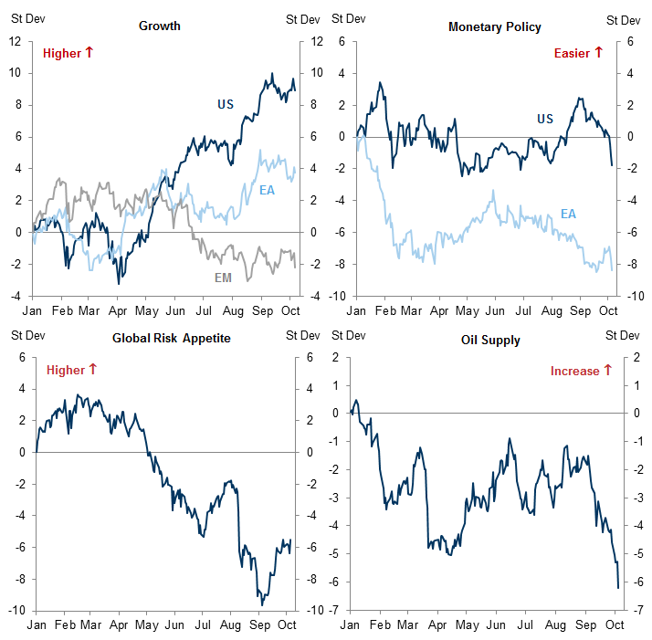
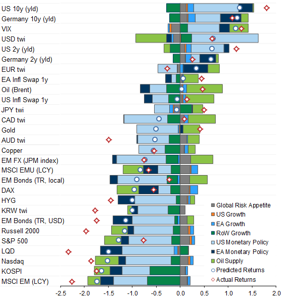
  • How our macro factors viewed last week. Monetary policy fears were clearly the biggest macro theme of the week. This theme was visible in the jump in US and German yields, but was further consistent with the weakness of risk assets, the rallies in USD and EUR TWIs, and the sharp declines in credit ETFs (LQD, HYG, EMB, and LEMB). The next most important macro themes of the week were “oil supply” and “EM growth”. Oil traded higher on the week due to what our model identified as supply concerns, but would have traded higher still had it not been for offsetting concerns about EM growth and DM monetary policy.

Distilling Macro Themes from Market Prices

Macro market volatility jumped this week, with the 10-year Treasury yield jumping 17 bps to close the week at 3.23% (its highest level since 2011), and Brent oil prices rising $3.57 at midweek before closing the week $1.44 higher at $84.26 (its highest level since 2014). Equities fell only modestly, but it was a terrible week for total returns in credit, with HYG dropping 1.3% (the most since February) and LQD falling 1.75% (the largest weekly drop since the fall of 2016).
Such large moves across markets naturally raise the question: What’s moving markets? In this Global Markets Analyst, we discuss some preliminary estimates of a macro factor model designed to answer such questions.[1] The goal of such models is to extract macro-themed statistical factors from market returns. This has long been the focus of our “Wavefront” baskets.[2]What is new about the approach described below is the modeling strategy, which is capable of extracting macro factors from a wide range of assets and asset classes. In our discussion below, we use these factors to show that last week’s market moves were dominated mainly by concerns about monetary tightening.
Economic factor models are structurally similar to factor models more generally. Their goal is to understand the pricing behavior of a very large cross section of assets using only a very small number of “macro factors”. What differentiates macro factors from statistical factors more generally is their correspondence to recognizable economic concepts like “US demand growth” or “global oil supply”. Most market participants have strong priors about how asset prices should respond to such shocks. For example, in response to market concerns about “US demand growth”, bond yields should rise, the US dollar should rise, equities should rally, and other indicators of “risk aversion” like the VIX, Japanese Yen, and credit spreads should drop. And since the shock originates in the US, the magnitudes of these responses should be larger for US assets than for their foreign counterparts. This logic generates a large cross section of “priors” about what a set of well-defined economic factors should look like. By imposing these priors during estimation, we’re able to back out factors that reflect market expectations of macro themes like US growth, European growth, global oil supply, etc.[3]
While the estimation procedure is non-trivial, the resulting economic factors are simple and easy to interpret. When our macro factors are used in regressions to explain the cross section of asset returns, the signs and magnitudes of the factor sensitivities (“betas”) are highly intuitive and consistent with economic priors. Importantly, this is true even for those factor loadings on which we do not impose priors (the majority of loadings). These regressions confirm the model’s ability to reveal the impact and influence of macro themes. While their relative importance varies by market, top-down macro themes like risk appetite, growth, monetary policy, and oil supply obviously feature centrally for equities, rates, credit, FX, commodities and their derivatives. Macro factors provide a lens for viewing and recognizing these themes.
Economic factors should not be confused with risk factors like “value” and “momentum”, which construct factors as long-short portfolios of assets sorted on their characteristics.[4] Nor should they be confused with pure statistical factors that are popular among risk managers for their ability to describe large covariance matrices. While these well-known factor models are useful for understanding the statistical properties of asset returns, neither is well-suited for understanding the macroeconomic drivers of returns. Our framework is designed to identify the latter, not the former.[5]
Our factors are closer cousins to “economic tracking portfolios”, which are portfolios of assets designed to track observable economic variables (like GDP growth, for example).[6] That said, there are some important (if nuanced) differences between our “macro factors” and “tracking portfolios”. Our factor definitions necessarily identify structural shocks, not their outcome. For example, a rise in the 2-year Treasury yield (an outcome) may reflect better growth momentum, or it may reflect tighter monetary policy. Tracking portfolios don’t shed any light on what’s causing the rate increase, they only reveal that rates should be rising. By contrast, our macro factors make it possible to decompose a rate move into its composite macro drivers (i.e., the structural shocks).
This structural character of our macro factors also implies a more stable relationship to market prices. To see why, consider inflation. During the 1980s, inflation expectations were the dominant driver of inflation. In this environment, higher inflation meant rate hikes were coming, hence equity betas to inflation were negative. Today, by contrast, inflation expectations are well-anchored, and growth expectations are the dominant driver of inflation. As a result, inflation surprises are a less signal of impending rate hikes than of growth, and equity betas to inflation are consequently more positive. This example illustrates how structural changes can undermine the stability of the statistical relationship between equities and inflation. At the same time, it sheds light on why the relationship of equities to the underlying shocks is stable: rate hike fears are always a negative for equities, while stronger growth expectations are always a positive. [7]

Macro factors from market prices

As explained above, the trick to extracting economic factors from market data is to recognize that common macro narratives (like “US monetary fears” or “oil supply concerns”) leave well-defined fingerprints in the cross-section of macro asset prices. For example, when markets are focused on monetary policy, say, around a hawkish-sounding Fed decision, it will generally be true that equities will trade lower while bond yields and the US Dollar move higher, with similar patterns visible in global assets. By contrast, if markets are worried, say, about a tightening of credit conditions in China, we will see a materially different fingerprint: equities will trade down (more so in EM Asia than in DM), global bonds will rally, and EM currencies with larger trade exposures to China will show more weakness against the Dollar. Of course, the daily flow of market pricing is never as clean as the above examples suggest, since markets are usually digesting several themes in parallel. Distilling the primary market narratives from market prices is a complex task.
Our model generates macro factors that are reverse engineered from patterns in market returns like those described above. To do this, we use Bayesian econometric techniques to impose “prior” views on the “beta” coefficients that quantify the impact of macro shocks on market outcomes.[8] In practice, these priors represent carefully articulated views about the signs and relative magnitudes of the factor loadings. We impose priors only where we have high conviction, and our experience thus far suggests that only a modest number of priors appears necessary to generate economically sensible “posterior” estimates for the full cross section of betas.
To estimate the model, we use weekly returns since 2012 for 28 major global assets to identify seven underlying economic shocks. These 28 assets are listed in the first column of Exhibit 1, and include 8 global equities (including the VIX), 6 global rates measures, US and UK inflation swaps, 2 US credit indices, 7 trade-weighted FX indices, and 3 commodity markets. Within equities, rates and FX, these assets are chosen to balance the regional representation among the US, Euro Area, and EM. Our model assumes these assets can be explained by a common underlying “factor structure” consisting of 7 major types of macroeconomic shocks (or “macro narratives”). These are listed across the top of Exhibit 1: one factor for global risk appetite, 3 factors for regional demand growth (US, Europe, and EM), 2 factors for monetary policy (Fed and ECB), and one factor for oil supply. This model could be estimated on daily data, but to reduce the potential problems introduced by the imperfect overlap of global information flow and trading hours, the model is estimated on weekly returns (and for bonds, weekly yield changes).
Exhibit 1 reports the beta coefficients for our 28 assets (note that the estimates here may differ from those in our previous Daily due to changes in our choice of assets and priors). To aid interpretation, the units on all factors and asset returns are scaled to a weekly standard deviation of one. Hence, the top-left cell in the table, for example, shows that a 1-sigma increase in “global risk appetite” is expected to cause a 0.6-sigma increase in the return on the S&P 500. Reading further down the column reveals that the magnitude of the market impact from a shift in “global risk appetite” is relatively uniform across equities, and coincidentally, is also relatively uniform across bond yields, FX indices, and oil prices. The assets with negative betas to global risk appetite are: US Investment Grade Credit (LQD), reflecting its high sensitivity to long-duration rates; the trade-weighted Dollar, Euro, and Yen, consistent with their well-known roles as safe-haven currencies; and the VIX, which obviously drops in response to “risk on”.[9]
The next three columns of Exhibit 1 describe the impact of “aggregate demand shocks” emanating from the US, Europe, and EM. To help the model disentangle regional growth from global risk appetite, we impose a “monotonicity” prior, to require that regional shocks have a larger impact on their local equity market than on foreign equities.[10] Consistent with our priors, a US demand shock in the estimated model sends global 10y yields higher, the US Dollar higher, EM FX lower, and oil prices higher. Analogous patterns are visible in the response to demand shocks from Europe and EM.
The next two columns of Exhibit 1 summarize the response to monetary shocks. An easing of monetary conditions by the Fed sends equities higher, bond yields higher (including EM – note that EMB and LEMB reflect total returns, not yields), inflation swaps higher, commodities higher, and the VIX lower. The US dollar and Euro both weaken in response to Fed and ECB easings, respectively, while all other currencies strengthen. Finally, in the next-to-last column of Exhibit 1, a positive shock to oil supply is bad for oil prices, good for equities, bad for US inflation swaps, good for the US Dollar, bad for the Canadian Dollar, bad for Gold and Copper, and a headwind for EM FX. All of these market reactions are consistent with our priors on the effects of monetary and oil supply “shocks”.

Exhibit 1: Model loadings (betas) of asset returns on economic factor returns

1. Model loadings (betas) of asset returns on economic factor returns. Data available on request.
Source: Goldman Sachs Global Investment Research
Exhibit 2 plots the 7 economic factors extracted from the model. The top-left panel plots the market-implied, cumulative shocks to US, European and EM growth expectations. Consistent with our general view of the macro market narrative in 2018, all three regions were tracking roughly in line with one another until April, following which growth expectations rose for the US, moved sideways for the EA, and fell for EM (“A ‘Growthy’ EM Correction”, Global Markets Daily, July 9, 2018). This expected growth divergence reached its peak in August but has since appeared to stabilize (and in our forecasts we expect to see re-convergence; “Keeping On Keeping On”, Global Views, September 23, 2018).
The second (top-right) panel of Exhibit 2 plots the market-implied, cumulative shocks to Fed and ECB monetary expectations. Note that these measures of “monetary tightening” differ materially from conventional measures like the 2-year rate. This is because these measures do not include current or expected moves in policy rates that are attributable to current or expected changes in the expected strength of economic growth (the latter which are shown in the first plot). Since we do not include an inflation factor in this version of the model, our measure of “monetary tightening” reflects changes in the market’s inflation view alongside changes in policy views per se. Consistent with this interpretation, the plot of US monetary views shows broad tightening during the first half of the year, coincident with headline CPI surging to 2.9% from 2.1% at the end of 2017, followed by a relaxation of these concerns as some inflation measures appeared to cool.
The third (bottom-left) panel of Exhibit 2 plots our measure of “Global Risk Appetite”. As noted above, the loadings reported in Exhibit 1 appear to check all the boxes for a “risk on, risk off” factor, at least with respect to sign restrictions. With respect to the relative magnitude of loadings, however, our priors are weaker for this factor than for the other six. We therefore interpret this factor with a corresponding degree of caution. What is risk appetite, and what drives it? In our view, the primary drivers obviously have mostly to do with shocks to expected future income and wealth. We also suspect these drivers are shaped to a meaningful degree by the funding and risk-taking capacity of financial intermediaries (notably global banks).[11] With this intuition in hand, it makes sense to us that the YTD change in risk appetite shown in Exhibit 2 has been roughly flat. In particular, the decline in risk appetite between April and August roughly corresponds to a period of disappointing growth expectations. The modest rally in risk sentiment this fall (and also to start the year) also map roughly to the ebb and flow of macro data surprises.

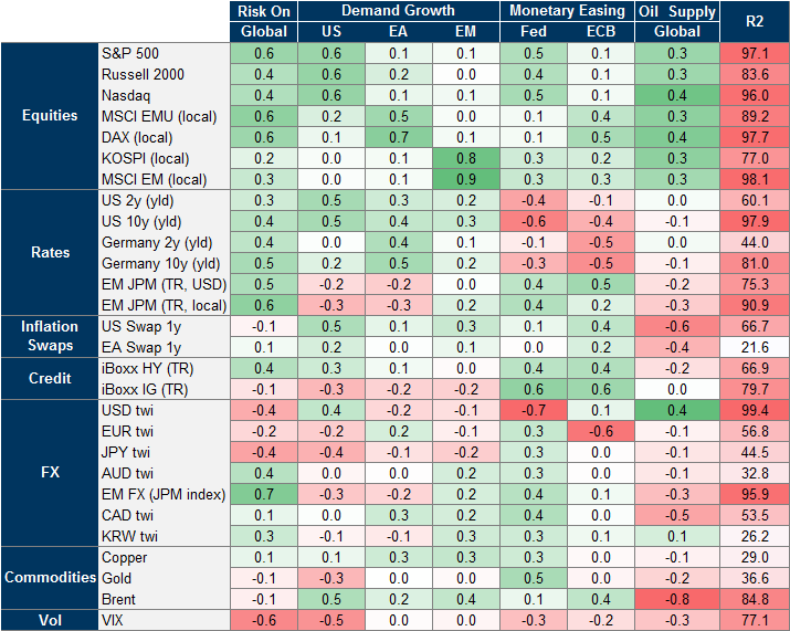
Exhibit 2: Economic Factors: Risk appetite, growth, policy and oil supply

2. Economic Factors: Risk appetite, growth, policy and oil supply. Data available on request.
Source: Goldman Sachs Global Investment Research
An interesting feature of “Global Risk Appetite” is that it doesn’t reflect the VIX spike in early February of this year. On its face, this is an affront: if any single asset is a surrogate for “Global Risk Appetite”, surely it’s the VIX. So how is it that this factor didn’t plunge in February? One obvious answer is that the VIX spike was a liquidity event, not a “risk off” event. As such, we are inclined to view the non-appearance of this event in our factor as a feature, not a flaw. But this then raises the question: Where does the VIX spike show up in the model, if not in global risk appetite? The answer is twofold. First, it shows up in the residual of the regression of VIX on the factors. Though this residual is not shown here, it is large and persistent during January and February. In our view, this is where it belongs: the VIX spike was more technical than fundamental.
Second, to the extent that the VIX spike shows up anywhere, it shows up in the factor for “US monetary policy”. This, too, makes some sense to us. While the VIX spike was obviously not the literal outcome of a policy tightening, its “fingerprints” were arguably similar. In particular, to the extent that the VIX spike might have caused temporary pressure on bank balance sheets, its fingerprint on financial markets would have been similar to a monetary tightening. While our views here are still developing, it does not seem unreasonable to us to assume that such “plumbing problems” might weigh on funding costs, and thus might be hard to distinguish from a monetary tightening (this is a topic for future research).
Finally, the fourth (bottom-right) panel of Exhibit 2 plots our “oil supply” factor. Consistent with this year’s 26% increase in the price of Brent, the oil supply factor shows a sizeable decline. While the oil demands implied by the regional growth factors also played a role, they were somewhat offsetting, so that supply concerns were clearly the dominant influence on market pricing. This supply narrative is broadly consistent with the views of our commodity team market concerns over the fall-out from oil sanctions on Iran (“Navigating a Sea of Uncertainties”, Commodities Research, October 4, 2018).

How our macro factors interpreted last week

We conclude our discussion by using our model to assess the macro drivers of last week’s jump in bond yields and sell-off in risk assets. Exhibit 3 provides a dense summary of the week-on-week repricing for the 28 assets included in our model. Assets are ranked in descending order by the magnitude of their model-predicted moves over the week. This ranks markets by the extent to which they were moving on macro concerns rather than idiosyncratic issues. The model-predicted moves are indicated by circles, whereas the actual market moves are indicated by diamonds. Note that yields are in changes, whereas most other assets, including the US credit and EM bond market indices, are in total returns. Note also that the units are calibrated to the weekly standard deviation of the actual changes for that asset. Model-predicted moves are further decomposed in to their constituent macro drivers, which for each asset are simply the 7 macro factors multiplied by their respective factor betas. These are illustrated using a stacked bar chart.

Exhibit 3: Factor decomposition of asset returns for week of October 1, 2018

3. Factor decomposition of asset returns for week of October 1, 2018. Data available on request.
Source: Goldman Sachs Global Investment Research
Monetary policy fears were clearly the biggest macro theme of the week. In “asset space”, this theme was visible in the jump in US and German yields. The monetary signal (as opposed to a growth signal) was confirmed by the behavior risk assets, which were mostly down on the week. It was also visible in the rallies in USD and EUR TWIs, as well as the sharp declines in credit ETFs (LQD, HYG, EMB, and LEMB), which are typically hard hit by monetary concerns due to their double exposure to both rates and risk.
After US and European monetary policy, the next most important macro themes of the week were “oil supply” and “EM growth”, in no particular order. Indeed, oil itself would have been even higher on supply concerns had it not been for the offsetting concerns about EM growth alongside concerns about US and EA monetary policy. In fact, the model-implied change in oil prices was roughly flat on the week, a view with which the oil market, too, increasingly agreed by week’s end. The oil supply theme also played a big role in constraining the move in USD TWI, which otherwise would have rallied harder on the Fed view.
Our sense from speaking with clients last week is that their interpretations of the market moves were in line with the broad strokes of the macro themes discussed above. But we also encountered a fair amount of confusion. There are weeks when a single macro theme stands out, but more often it is the case that multiple themes are at play. During “macro heavy” weeks like last week, considerable effort may be required to discern and disentangle these cross currents. As Exhibits 2 and 3 hopefully persuade, a macro factor model can greatly assist this task.

Charlie Himmelberg

Matthieu Droumaguet

James Weldon

The authors would also like to thank Julian Richers for his contributions to this report.
  1. 1 ^ See also our previous report, “An Economic Factor View of EM Equities”, Global Markets Daily, Sept. 27, 2018.
  2. 2 ^ “Wavefronts 2.0: The impact of macroeconomic shocks on markets”, Global Economics Paper No. 228, Jan. 31, 2016.
  3. 3 ^ We use Bayesian econometrics to impose our economic priors on the factor loadings. Our Bayesian approach provides a natural way to impose such priors. It also allows us to assume time-varying volatility for both the factors and idiosyncratic error terms. Allowing for the latter allows for a more realistic description of market returns – the volatilities of both macro themes and asset-specific returns obviously vary over time – appears to improve the fit of the model.
  4. 4 ^ The ever-growing popularity of characteristic-based “risk factors” like “value” and “momentum”, for example, reflects that these factors are known to offer risk premia with desirable risk-reward properties (for example, see “Value and Momentum Everywhere”, by Clifford Asness, Tobias J. Moskowitz, and Lasse Heje Pedersen, Jan. 30, 2018, Journal of Finance, 68(3)). There has also been recent revival of an older academic literature on macro pricing factors which dates back to Nai-Fu Chen, Richard Roll, and Stephen A. Ross (1986), “Economic Forces and the Stock Market”, Journal of Business, 59, 383-403. But these factors are designed to identify risk premia, not macro themes.
  5. 5 ^ This is not to rule out the possibility that risk factors and macro factors may be related in some interesting ways. Indeed, our inclusion of a “Global Risk Factor” in our list of macro factors reflects our belief that shocks to risk appetite are drivers of asset returns which are distinct from macro shocks.
  6. 6 ^ See “Economic Tracking Portfolios”, by Owen Lamont, Journal of Econometrics, 105(1), pp. 161-184.
  7. 7 ^ In an earlier effort to extract “macro views from market data”, we pursued a strategy that was essentially identical in spirit to Lamont (2001), namely, we designed market factors that explicitly aimed to track economic outcomes like GDP growth and inflation (“Tracking Macro Views in Market Data”, Global Markets Analyst, April 3, 2018). Over the course of that research, however, we came to recognize that the construction of such portfolios is complicated by the structural instabilities described in the text. The design of the macro factors described here effectively sidesteps this issue.
  8. 8 ^ This is similar to the method of “sign restrictions”, which is increasingly popular among academic macroeconomists. See for example, “Sign Restrictions in Structural Vector Autoregressions: A Critical Review”, by Renée Fry and Adrian Pagan, Journal of Economic Literature, Dec. 2001, 49(4), pp. 938-60. For a related applications to financial market data, see also “The Economic Impact of the New Oil Order on Emerging Asia”, Asia Economics Analyst, Jan. 12, 2015; and “Oil Supply versus Demand: A Market Perspective”, US Daily, Feb. 10, 2015.
  9. 9 ^ For a more in-depth analysis of risk sensitivities across FX, see “Explaining risk correlations across DM and EM exchange rates”, EM Macro Themes, Aug. 11, 2018.
  10. 10 ^ This generates more reasonable results than the approach used in our previous Daily, which imposed zero restrictions on the cross-region impact of regional shocks.
  11. 11 ^ See “Financial intermediaries and the cross-section of asset returns”, by Tobias Adrian, Erkko Etula, and Tyler Muir, 2014, Journal of Finance LXIX, 2557-2596.

Investors should consider this report as only a single factor in making their investment decision. For Reg AC certification and other important disclosures, see the Disclosure Appendix, or go to www.gs.com/research/hedge.html.