- Intro
- Forecasting long-term S&P 500 returns
- Investment implications
- Outlook for aggregate vs. equal-weight performance
- How our long-term equity return forecast compares with consensus
- Considerations for portfolio managers with long investment horizons
- Appendix A: Components of our long-term equity return model
- Appendix B: Risks to our forecast
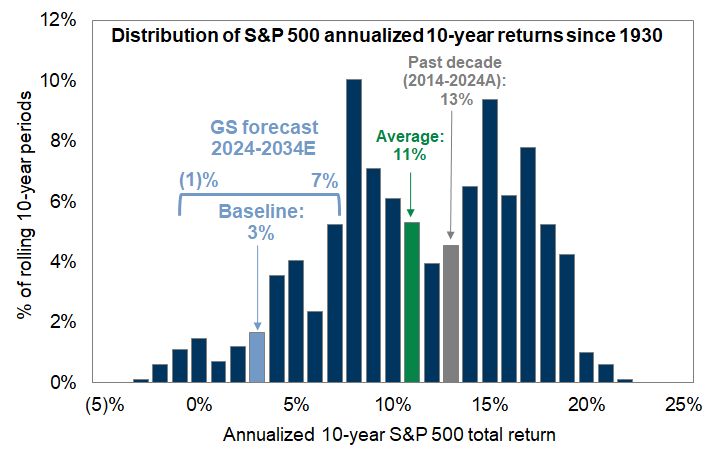
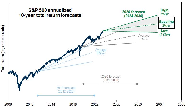
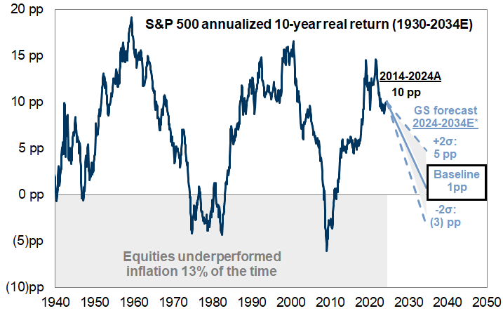
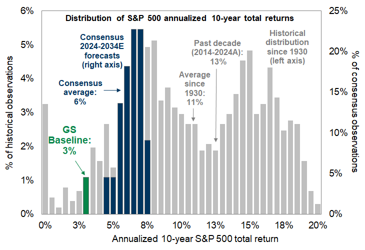
We estimate the S&P 500 will deliver an annualized nominal total return of 3% during the next 10 years (7th percentile since 1930) and roughly 1% on a real basis. Annualized nominal returns between -1% and +7% represents a range of likely outcomes around our baseline forecast and reflects the uncertainty inherent in forecasting the future. During the past decade the S&P 500 posted a 13% annualized total return (58th percentile).
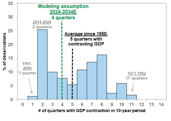
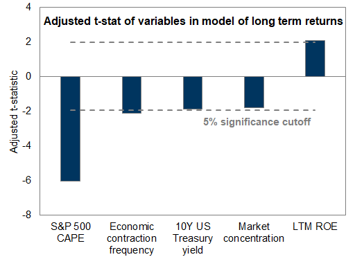
We model prospective long-term equity returns as a function of five variables: (1) starting absolute valuation, (2) stock market concentration, (3) economic contraction frequency, (4) corporate profitability, and (5) interest rates.
Our forecast would be 4 pp greater than our baseline if we exclude a variable for market concentration that currently ranks near the highest level in 100 years. The 7% return would rank in the 22nd historical percentile.
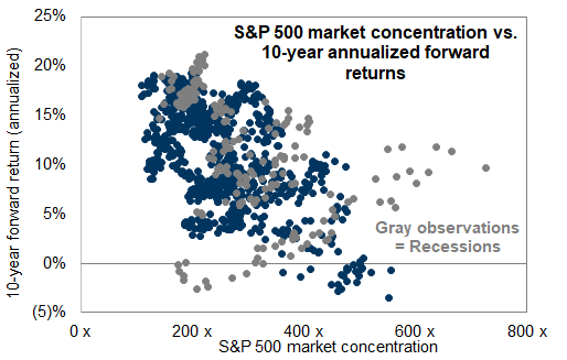
The intuition for why concentration matters for long-term returns relates to growth in addition to valuation. Our historical analyses show that it is extremely difficult for any firm to maintain high levels of sales growth and profit margins over sustained periods of time. The same issue plagues a highly concentrated index. Furthermore, the risk embedded in high concentration markets is not always reflected in valuation.
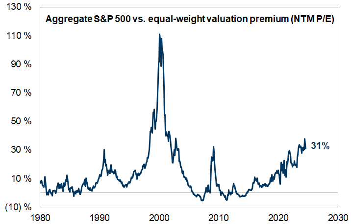
We expect the return structure of the stock market will broaden in the future. Today's extremely high market concentration suggests that the S&P 500 equal-weight benchmark (SPW) is likely to outperform the cap-weighted aggregate index (SPX) during the next decade by an annualized 200 bp-800 bp.
Our forecast suggests equities will face stiff competition from other assets during the next decade. Our 3% annualized equity return forecast combined with a current ten-year US Treasury yield of 4% and ten-year breakeven inflation of 2.2% suggests the S&P 500 has roughly a 72% probability of trailing bonds and a 33% likelihood of lagging inflation through 2034. Excluding concentration, the probabilities of underperforming would be 7% and 1%, respectively.
Our S&P 500 baseline 10-year return forecast is lower than the estimates of other market participants. Buy- and sell-side projections of the long-term return of US stocks averages 6% (range of 4% to 7%).
Forecasting long-term S&P 500 returns
Exhibit 1: S&P 500 annualized trailing 10-year returns: modeled vs. realized (1930-2024) and forecast (2024-34E)
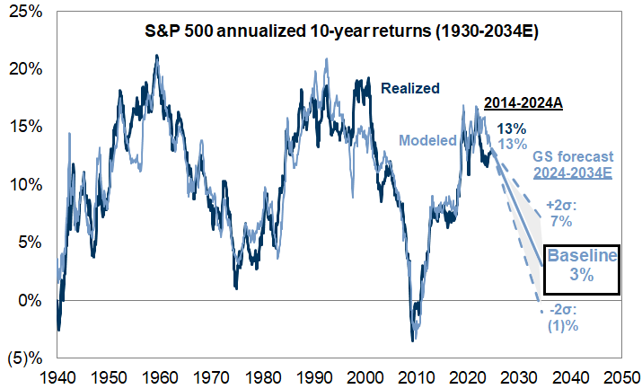
Exhibit 2: Distribution of S&P 500 annualized 10-year total returns, 1930-2024
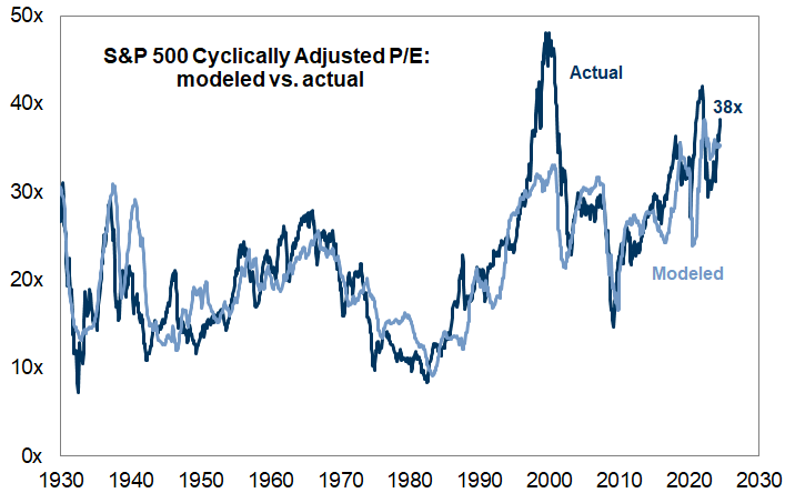
Valuation: S&P 500 cyclically adjusted P/E multiple (CAPE)
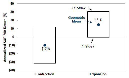
Economic fundamentals: Economic contraction frequency
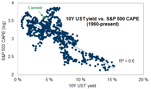
Interest rates: 10-year US Treasury yield
Market concentration: Ratio of the market cap of the largest-cap stock vs. the 75th percentile stock
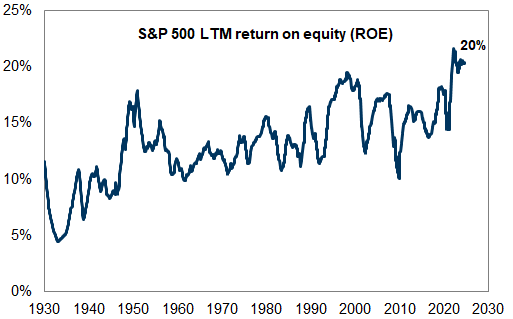
Profitability: LTM S&P 500 return on equity (ROE)
Exhibit 3: Details behind our regression model of S&P 500 10-year forward returns
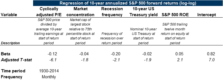
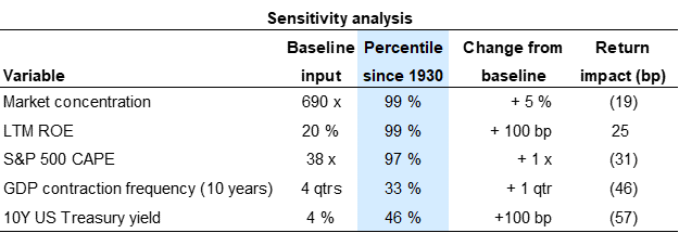
Exhibit 4: Sensitivity analysis around our baseline long-term US equity return forecast
Valuation
Exhibit 5: Episodes exist when valuations are stretched relative to fundamental and macro variables
Market Concentration
Exhibit 6: Annualized S&P 500 total return with and without market concentration variable
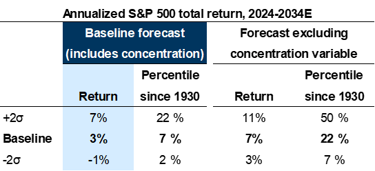
Exhibit 7: The 10 largest stocks in the S&P 500 account for more than a third of total market cap
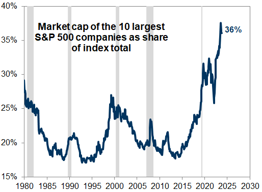
Exhibit 8: US equity market concentration 1925-2024
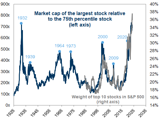
Exhibit 9: Valuation is not a perfect predictor of market concentration
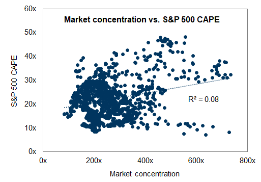
Exhibit 10: Relationship between concentration and valuation shifts over time
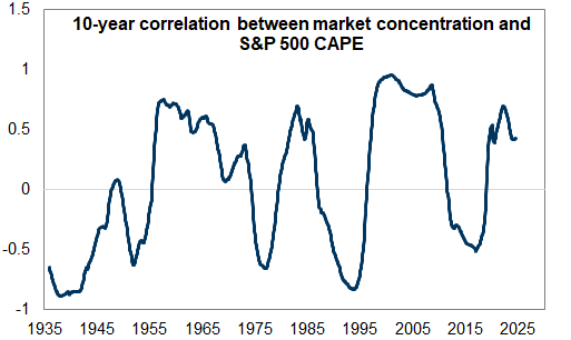
Exhibit 11: Higher starting market concentration associated with higher volatility
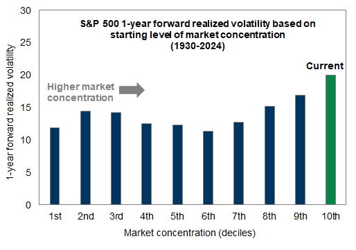
Exhibit 12: Outside of recessions higher market concentration is associated with lower forward returns

Exhibit 13: Absolute valuations for top 10 and remaining S&P 500 stocks over time
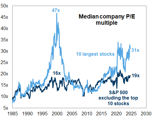
Exhibit 14: Yield gaps for top 10 and remaining S&P 500 stocks over time
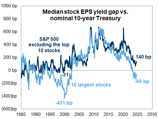
Exhibit 15: Maintaining rapid sales growth for 10 consecutive years is rare
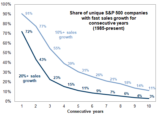
Exhibit 16: Maintaining high levels of profitability for 10 consecutive years is also challenging
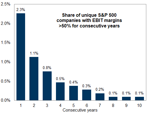
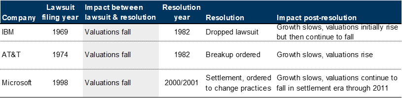
Exhibit 17: Historical examples of regulatory scrutiny
Economic contraction frequency
Exhibit 18: Frequency of economic contractions in rolling 40-quarter (10-year) periods since 1950
Risks to our forecast
Exhibit 19: Our S&P 500 annualized 10-year total return forecasts: 2012 vs. 2020 vs. 2024
Investment implications
Exhibit 20: Distribution of S&P 500 annualized 10-year return forecast, 2024-2034E
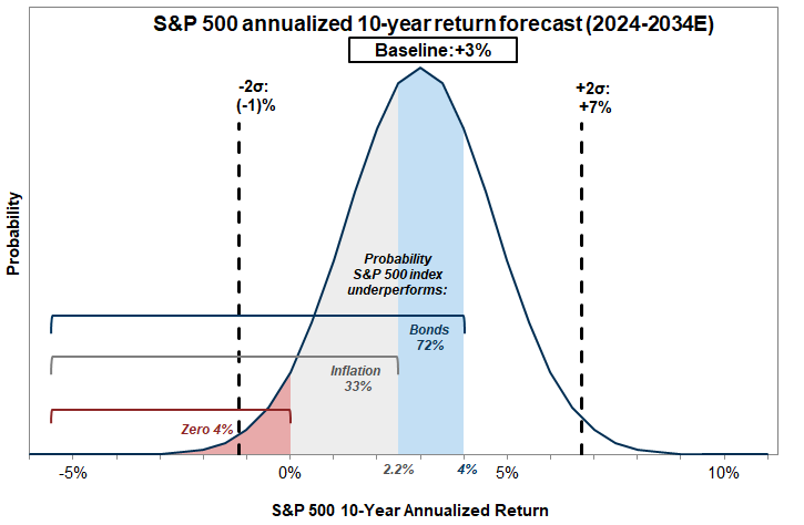
Exhibit 21: Relative 10-year performance of equities vs. bonds
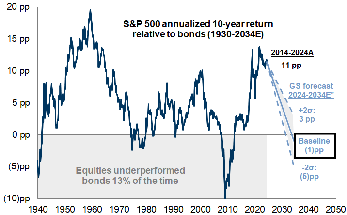
Exhibit 22: Relative performance of equities and inflation
Outlook for aggregate vs. equal-weight performance
Exhibit 23: Equal-weight S&P 500 has typically outperformed the aggregate index
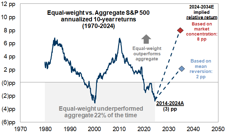
Exhibit 24: Higher market concentration implies future outperformance of low market cap vs. high market cap stocks
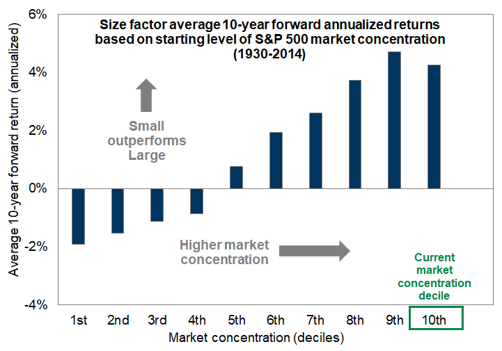
Exhibit 25: The current high level of market concentration suggests the equal-weight S&P 500 will outperform the aggregate index by an annualized 8 pp during the next decade
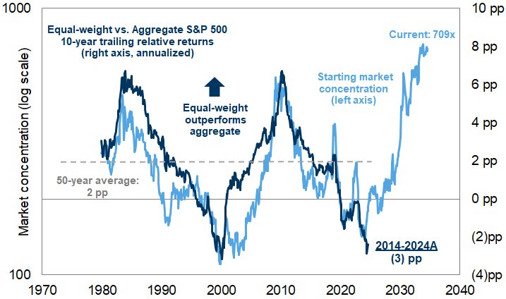
Exhibit 26: The aggregate S&P 500 trades at a 31% valuation premium to the equal-weight index
How our long-term equity return forecast compares with consensus
Exhibit 27: Goldman Sachs vs. consensus long-term US equity return forecasts
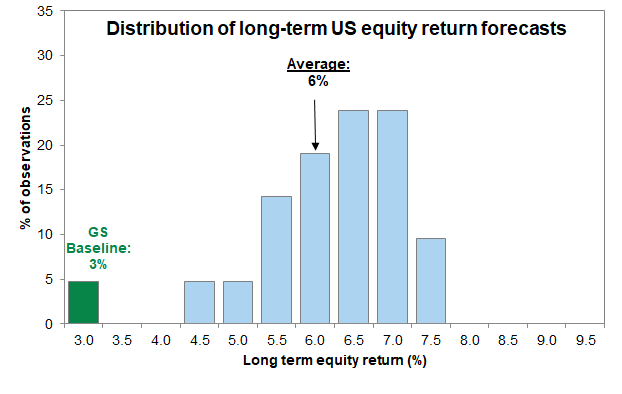
Exhibit 28: Goldman Sachs and consensus forecast the S&P 500 index will deliver a below-average annualized return during the next decade
Considerations for portfolio managers with long investment horizons
Exhibit 29: Corporate pension plan long-term annualized return assumptions
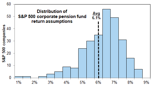
Exhibit 30: Public pension plan return assumptions
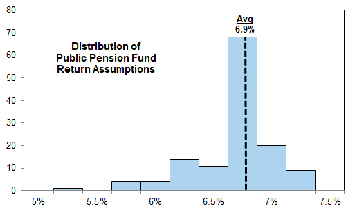
Exhibit 31: Asset allocation among corporate pension funds
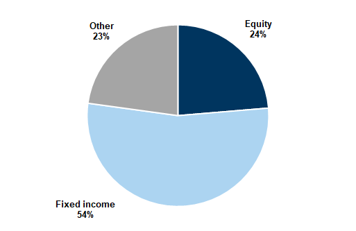
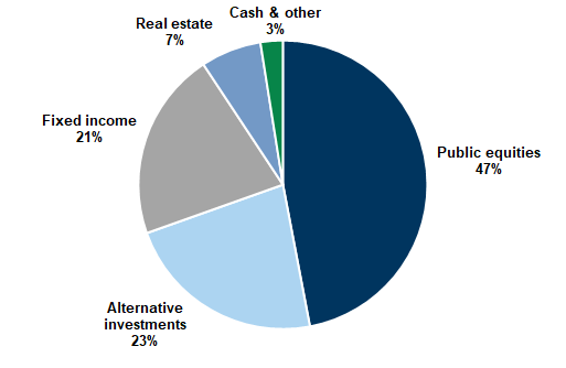
Exhibit 32: Asset allocation among public pension funds
Appendix A: Components of our long-term equity return model
Components of our long-term return forecast model
Valuation: S&P 500 cyclically adjusted P/E multiple (CAPE)
Economic fundamentals: Economic contraction frequency
Interest rates: 10 year US Treasury yield
Market concentration: Ratio of the market cap of the largest-cap stock vs. the 75th percentile stock
Profitability: LTM S&P 500 return on equity (ROE)
Exhibit 33: Starting valuation is the most important variable in helping explain forward returns
Valuation
Exhibit 34: S&P 500 Cyclically-adjusted P/E ratio
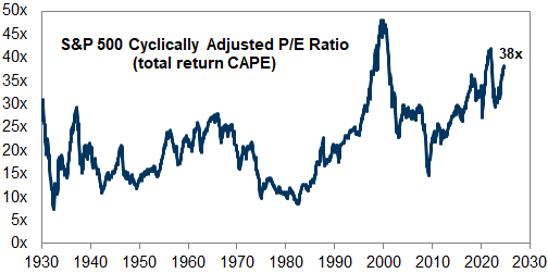
Exhibit 35: Historical distribution of S&P 500 CAPE multiples
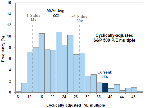
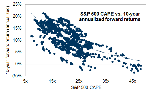
Exhibit 36: 10-year annualized S&P 500 returns based on valuation at initial investment
Economic contraction frequency
Exhibit 37: Frequency of economic contractions in rolling 40-quarter (10-year) periods since 1950
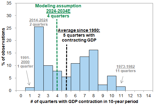
Exhibit 38: Distribution of annualized total returns during economic expansion vs. contraction
Interest Rates
Exhibit 39: Nominal 10-year US Treasury yields, 1930-2024
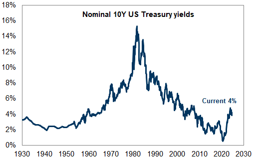
Exhibit 40: Valuations are inversely related to interest rates
Market Concentration
Exhibit 41: Market concentration over time
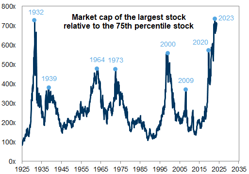
Exhibit 42: Outside of recessions higher market concentration is associated with lower forward returns
Profitability
Exhibit 43: S&P 500 LTM ROE
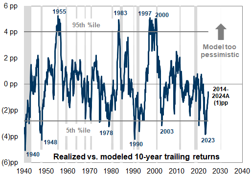
Historical periods where our model fails to explain returns
Exhibit 44: Difference between actual and modeled long-term returns
Appendix B: Risks to our forecast
Exhibit 45: 36% of S&P 500 constituents turnover during the typical 10-year period
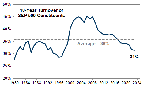
Exhibit 46: Historical 10-year annual productivity
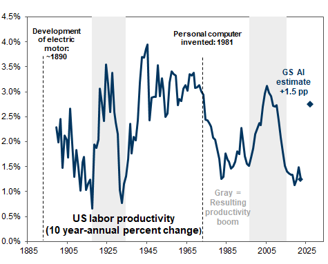
Exhibit 47: US household allocations to equities are at all-time highs
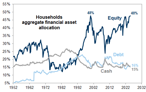
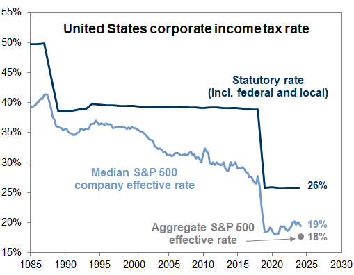
Exhibit 48: S&P 500 companies' tax rate has declined over the past several decades
Investors should consider this report as only a single factor in making their investment decision. For Reg AC certification and other important disclosures, see the Disclosure Appendix, or go to www.gs.com/research/hedge.html.